
Table of Contents
Introduction
This project tackles a classic linear controls problem: balancing an inherently unstable system, and making the system robust to physical disturbances. Taking inspiration from the rather impressive Cubli robot, a 15cm cube capable of jumping up to balance on an edge or a corner, I set out to design a cube capable of stabilizing itself on an edge. While the corner and jumping techniques of the Cubli are interesting, I would be more interested in continuing this project in an adaptive control direction, potentially making the cube robust to changes in center of mass (perhaps by adding weights to the corners during operation). Over the course of a semester, mechanical, mechatronic, and control designs were implemented, and the resulting system was quite robust to external disturbances. The CAD, code, and technical reports for this project are located in a Github repo, here.
System Modeling
Because the cube is being balanced on an edge, it only needs to be modeled in two dimensions. The FBD for the cube is shown:
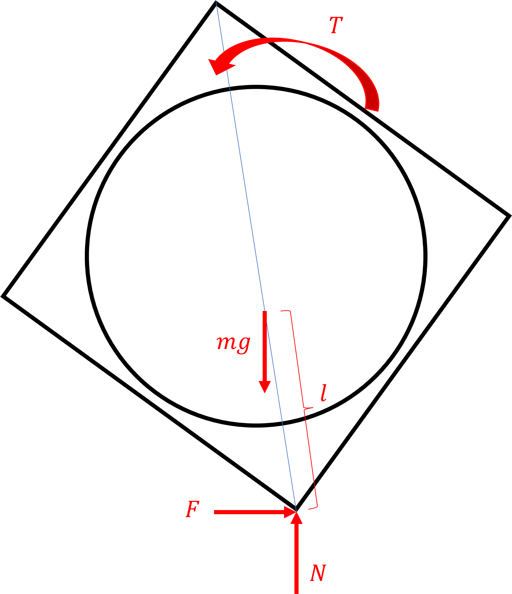
The main forces to consider are the forces of gravity on the cube (mg, applied at a distance l to the center of mass from the pivot point), the reaction forces at the ground (N and F), the torque applied by the motor (T), and the damping forces at the wheel and the cube (not drawn, velocity dependent). The equations of motion can be written:
\(\sum{M_c^o}=(m_w + m_c)l_csin(\theta_c)+T+C(\dot\theta_w - \dot\theta_c)=I_c^o\ddot\theta_c\) \(\sum{M_w}=T-C(\dot\theta_c - \dot\theta_w)=I_w\ddot\theta_w\)
The inertia properties were approximated from theory by treating the cube as composed of one-dimensional rods, the wheel as a ring, and the battery as a rectangular prism. Moments of inertia were transformed to the relevant axis by the parallel axis theorem.
To simplify the controller design, the damping characteristics of the system were considered to be negligible. This decouples the two governing equations, which are no longer dependent upon one another. A single equation now needs to be controlled:
\(I_c^o\ddot\theta_c=(m_w + m_c)l_csin(\theta_c)+T\)
Linearizing this equation about the operating point $(\theta_c=0)$ using $sin(\theta)\approx \theta$ gives:
\(I_c^o\ddot\theta_c=(m_w + m_c)l_c\theta_c+T\)
For controller design, this is expressed in state space as:
\(\begin{bmatrix}
\dot\theta_c \\
\ddot\theta_c
\end{bmatrix} =
\begin{bmatrix}
0 & 1 \\ a & 0
\end{bmatrix}\begin{bmatrix}
\theta_c \\ \dot\theta_c
\end{bmatrix} + \begin{bmatrix}
0 \\ b
\end{bmatrix} T\)
Where $a = \frac{(m_w + m_c) l_c}{I_c^o}$ and $b = \frac{1}{I_c^o}$.
System Design
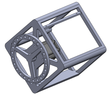
The mechanical system is designed in SolidWorks, and is composed of two primary 3D printed parts, the frame and wheel. The wheel is manufactured to have an adjustable mass, where bolts and nuts are added around the circumference in a symmetric fashion to increase or decrease the wheel inertia. Larger inertia of the wheel allows a higher torque to generate less acceleration of the wheel, increasing the time over which torque can be applied before hitting saturation limits on the motor; however, this also increases the magnitude of the gravitation torque destabilizing the system. The system mass was chosen somewhat arbitrarily and worked well. CAD files are included in the project’s GitHub repo.
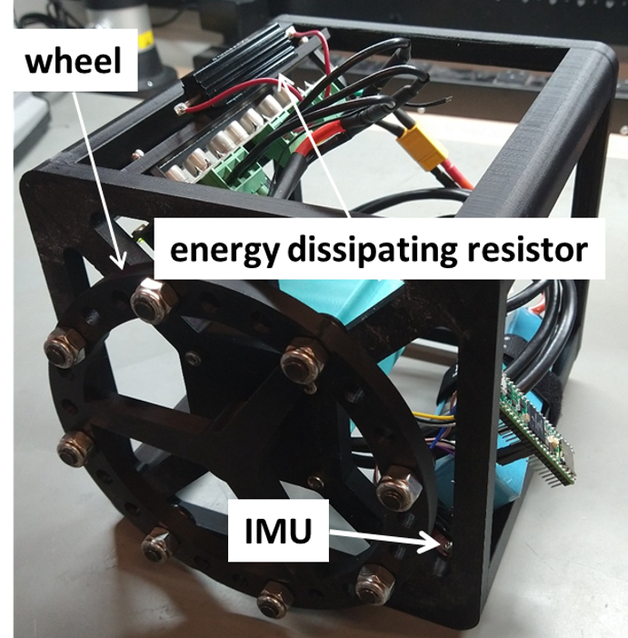
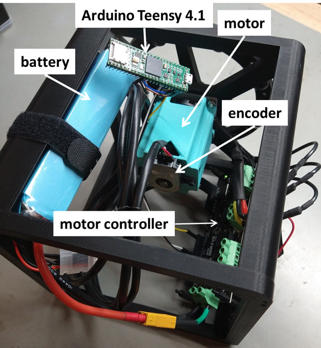
The mechatronic design for this system was similarly straightforward and simple. An IMU is used to determine orientation, which is placed near the pivot point to minimize the impact of linear accelerations on the complementary filter which is used to estimate orientation. An ODrive motor controller, motor, and motor encoder are used to apply torque to the system, and a Teensy microcontroller runs the control system. The system is powered by a LiPo battery, which is placed near the pivot point to minimize it’s destabilizing torque. A complete parts list is given below:
- Teensy 4.1 Microcontroller (Amazon)
- ODrive v3.6 Motor Controller (ODrive Shop)
- D5065 270kv Dual Shaft Motor (ODrive Shop)
- 20480 CPR Encoder (ODrive Shop)
- ICM 20480 IMU (Sparkfun)
- 3300mAh 14.8V (4S) 100C LiPo Battery (Amazon)
System Control
State Observation
To design a state space controller, the entire state information must be accessible. To do this, partial observer is designed, the complementary filter, to combine acceleration and angular velocity measurements from the IMU into an estimate of the cube’s orientation. Two methods exist to estimate orientation from the IMU: integration of angular velocity, and the geometry of the gravity vector, shown in the equations below. Both equations reference the quantities shown in the figure below.
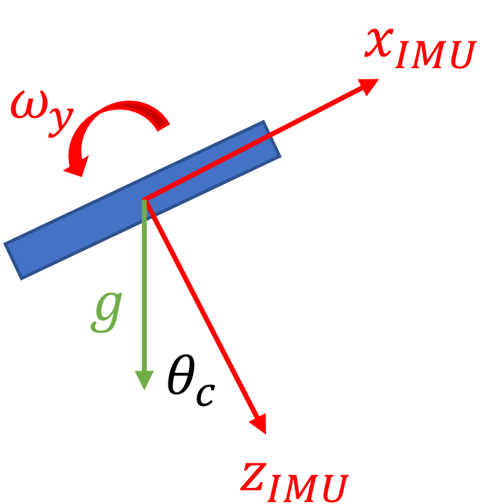 \(\theta^i_{c,gyro}=\theta^{i-1}_c + \omega_y \Delta t\)
\(\theta^i_{c,accel}=tan^{-1}{\frac{a_x}{a_z}}\)
Because gyroscope measurements are prone to drift, the gyroscope method is accurate in the short term, and tracks high frequency movements well; however, its long-term accuracy and low-frequency characteristics are poor. Conversely, the acceleration method tracks low-frequency movements well, and
has good long-term accuracy. The complementary filter combines both estimates in an infinite-impulse response filter, given below:
\(\theta^i_c=\alpha \theta^i_{c,gyro} + (1 - \alpha)\theta^i_{c,accel}\quad 0 \ll \alpha < 1\)
With this computation, the entire system state is estimated, as $\dot\theta_c=\omega_y$ is observed directly.
\(\theta^i_{c,gyro}=\theta^{i-1}_c + \omega_y \Delta t\)
\(\theta^i_{c,accel}=tan^{-1}{\frac{a_x}{a_z}}\)
Because gyroscope measurements are prone to drift, the gyroscope method is accurate in the short term, and tracks high frequency movements well; however, its long-term accuracy and low-frequency characteristics are poor. Conversely, the acceleration method tracks low-frequency movements well, and
has good long-term accuracy. The complementary filter combines both estimates in an infinite-impulse response filter, given below:
\(\theta^i_c=\alpha \theta^i_{c,gyro} + (1 - \alpha)\theta^i_{c,accel}\quad 0 \ll \alpha < 1\)
With this computation, the entire system state is estimated, as $\dot\theta_c=\omega_y$ is observed directly.
Controller Design: Pole Placement via State Space
Before designing the state space controller, controllability must be checked:
\(C_m = \begin{bmatrix}B & AB\end{bmatrix} = \begin{bmatrix}0 & b \\ b & 0\end{bmatrix} \rightarrow Full Rank, Controllable\)
Time specifications are given by desired system characteristics, at settling time of $t_s = 1$ and a maximum overshoot of $M_p = 0.05 = 5%$:
\(M_p = 0.05 \rightarrow \zeta = \frac{-ln(M_p)}{\sqrt{\pi^2 + ln^2(M_p)}}=0.69\)
\(t_s = 1\rightarrow\omega_n=\frac{4}{t_s\zeta}=5.79\)
These metrics determine the system’s closed loop characteristic equation:
\(s^2 + 2\omega_n\zeta s + \omega_n^2=s^2+8s + 33.5960\)
The poles of the closed loop system can be placed accordingly:
\(det(sI - (A-BK))=|\begin{bmatrix}s & -1 \\ -a + k_1 b & s + k_2 b\end{bmatrix}|=0\)
\(s^2 + k_2 b s + a - k_1 b = s^2 + 8s + 33.5960\)
\(k_1 = 2.29\quad k_2 = 0.201\)
A few details of the controller implementation deserve notes. First, due to wires, and asymmetry, the center of mass of the device is slightly misaligned with the z-axis of the IMU, as shown in the figure below.
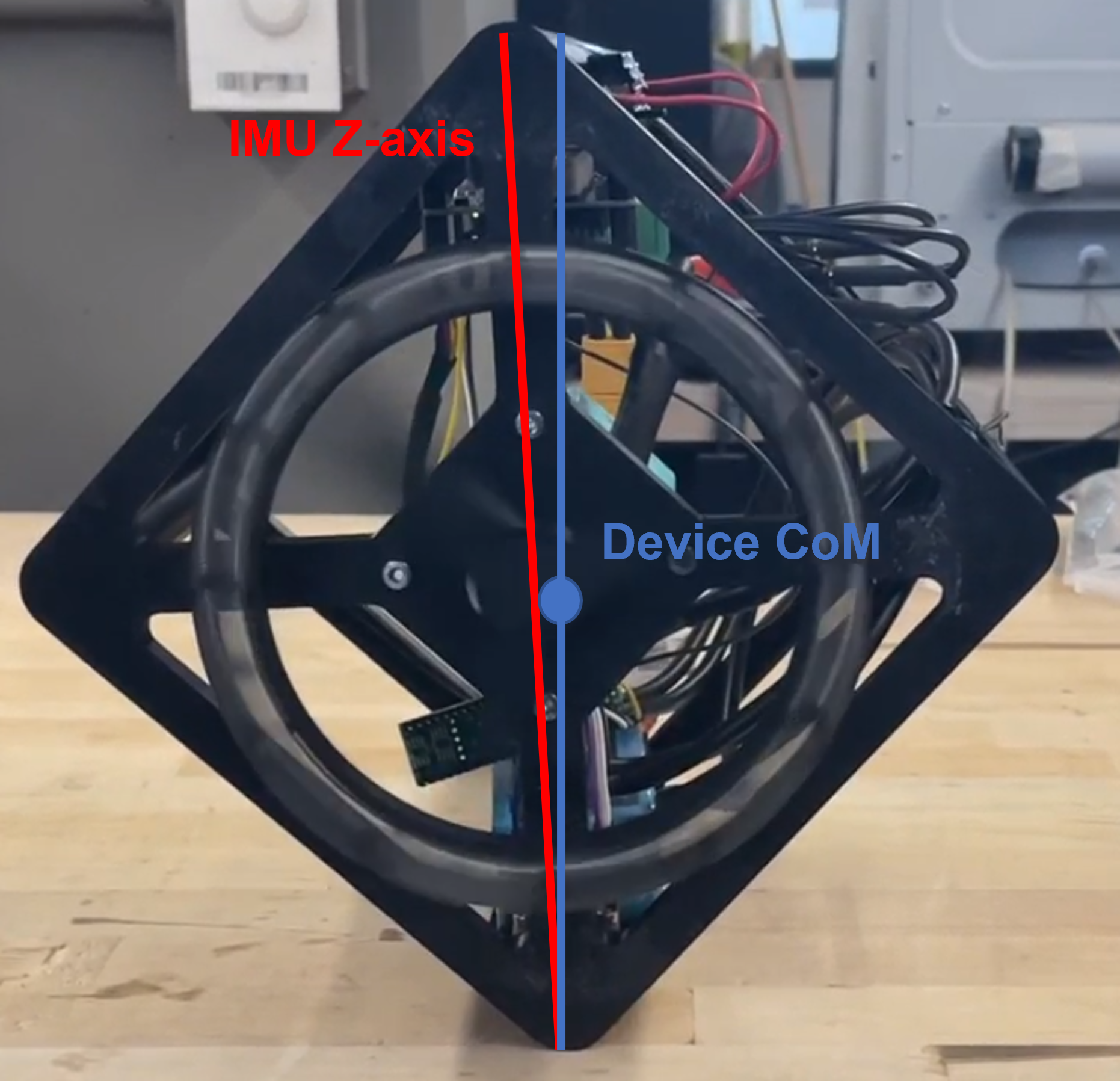 To correct for this, the device is balanced by hand, and this offset angle is measured. The offset can then be subtracted so that the device balances over its center of mass instead of the IMU Z axis. Secondly, the control loop is implemented at a rate of 200Hz. It is assumed that this is a sufficiently fast update rate to ignore the discrete control aspects of the controller and treat it as continuous.
Performance
Performance is perhaps most enjoyably evaluated by simply watching videos:
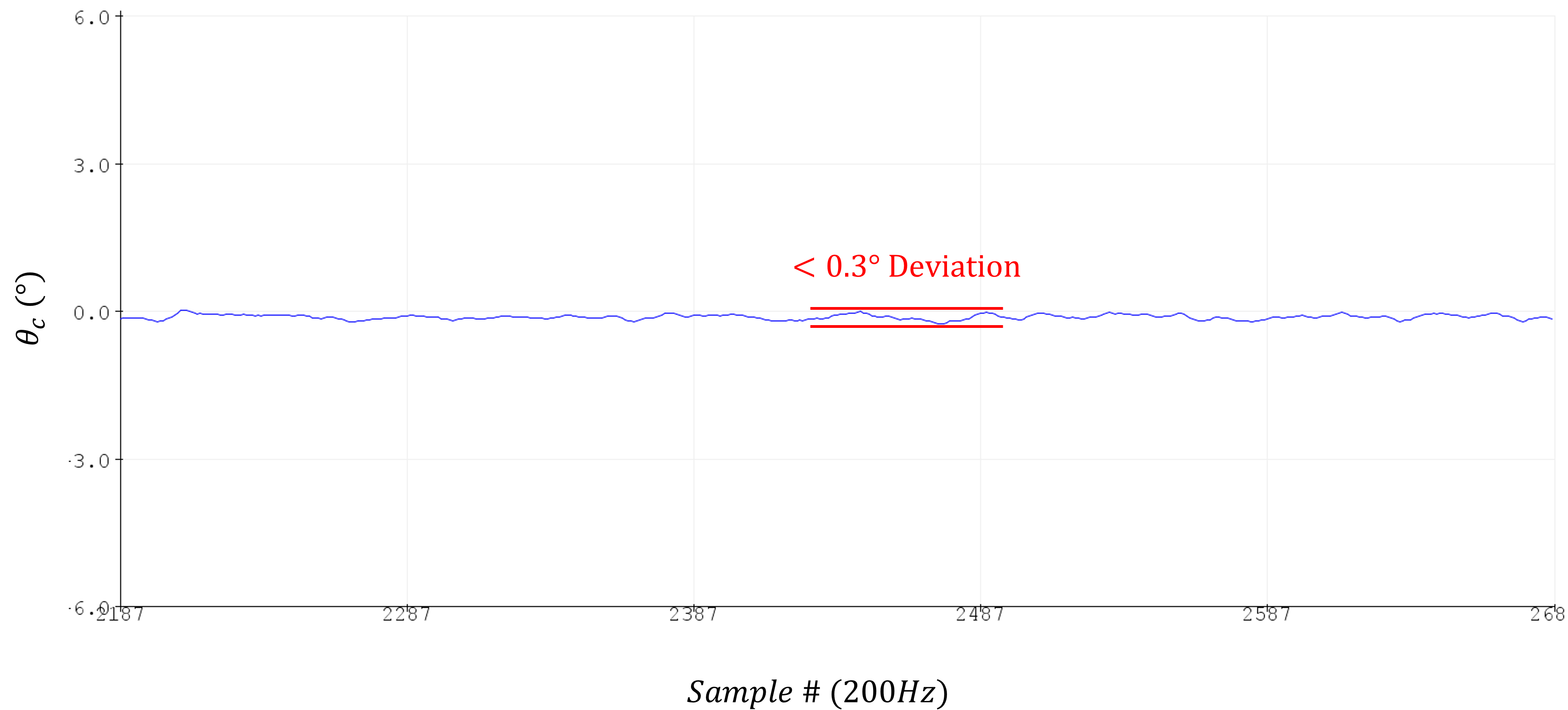
For more quantitative metric, consider the steady state operation, which maintains a deviation of less than $0.3\degree$.
 When rejecting a sizable disturbance, the following response was generated, with a settling time of 1.6s:
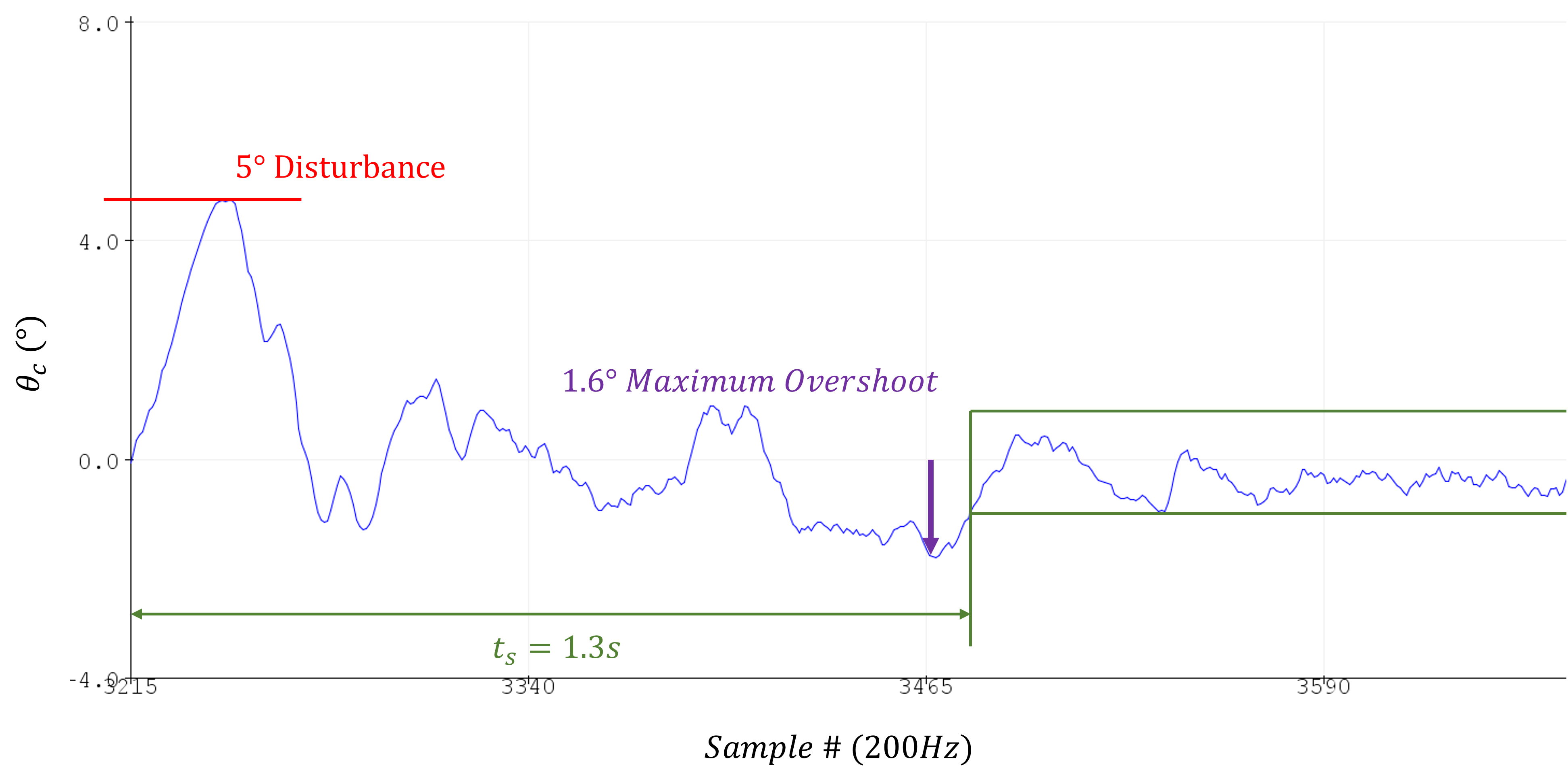 Overall, the cube is quite stable.
The main performance limitation is the fact that the speed of the cube’s wheel is not being controlled. Because of this, repeated perturbations in one direction will repeatedly accelerate the wheel in the same direction. After only a few such perturbations, the speed of the motor will saturate, and the motor will no longer be able to deliver torque to correct for further disturbance. This is easily corrected by regulating the wheel speed to zero as well; however, in order for this system to be controllable, the damping between the frame and wheel must be accurately characterized. An initial look at this damping shows it to be quite nonlinear, which will make this problem much more difficult.
Conclusion
The results of this project were quite strong. The project was a very straightforward application of linear control techniques, and balancing was achieved quickly and with no parameter tuning. In the future, I would like to target regulating the wheel velocity to zero, and potentially look into adaptive control methods which estimate the position of the center of mass in real time, and can adapt to changes, such as adding masses to one side of the cube.