
Table of Contents
Overview
Reconnaissance Blind Multichess (RBMC) is a chess variant where the opponent’s pieces are hidden from the player except for a 3x3 section of the board the player can sense before moving a piece. The game was developed at Johns Hopskins (website here), for use in artificial intelligence research. RBMC has several features which make it well suited to AI research: it involves imperfect information, long-term strategy, and little to no guiding common knowledge. RBMC is a Partially-Observable Markov Decision Process, where true game states are hidden, sensing and move results constitute observations, and moves are actions. There are effectively two AI approaches to this problem: the first involves tracking a belief state, reducing the belief state to regular chess, and using existing chess knowledge or techniques to guide move selection. However, classical chess evaluations do not take into account the significant differences between classical chess and RBMC, and therefore do not understand any strategy specific to RMBC. A second, and more powerful, approach attempts to learn strategy unique to RBMC (perhaps through self-play). My approach takes the first (and less powerful) approach, although I am interested in looking more into learning-based methods in the future. The code for this project is available here.
Rules
RBMC generally follows the rules of regular chess, with a few exceptions summarized from here for the reader’s convenience).
- A player cannot see where the opponent’s pieces are.
- Prior to making each move a player selects a 3 x 3 square of the chess board. It learns of all pieces and their types within that square. The opponent is not informed about where he sensed.
- If an agent captures a piece, it is informed that it made a capture (but he is not informed about what it captured).
- If a player’s piece is captured, he is informed that his piece on the relevant square was captured (but he is not informed about what captured it).
- There is no notion of check or mate (since neither player may be aware of any check relationship).
- A player wins by capturing the opponent’s king or when the opponent runs out of time. Each player begins with a cumulative 15-minute clock to make all her moves, and gains 5 seconds on that clock after each turn.
- A game is automatically declared a draw after 50 turns without a pawn move or capture. This mirrors the 50-move rule in chess, except here neither player needs to claim the draw for the game to end.
- If a player tries to move a sliding piece through an opponent’s piece, the opponent’s piece is captured and the moved piece is stopped where the capture occurred. The moving player is notified of the square where his piece landed, and both players are notified of the capture as stated above.
- If a player attempts to make an illegal pawn attack or pawn forward-move or castle, he is notified that the move did not succeed and his move is over. Castling through check is allowed, however, as the notion of check is removed.
- There is a “pass” move, where a player can move nothing.
Methods
My AI agent uses a particle filter to maintain a belief state regarding the existing board. It chooses sensing locations to maximize information gain (measured by entropy) while prioritizing threatening or weak squares in the belief state. Lastly, it selects moves using minimax search with alpha/beta pruning, performed and averaged over a number of the most likely boards. The python-chess library is used for managing the chess aspects of the game. For discussion of the methods, it will be assumed that my agent is playing white, for simplicity. The black methods are completely analogous, with the exception of the first move.
Belief State
The belief state is approximated by a particle filter which maintains $N$ individual chess boards. At the beginning of the game, the board is known exactly. After the first move, black has 20 available moves to make:
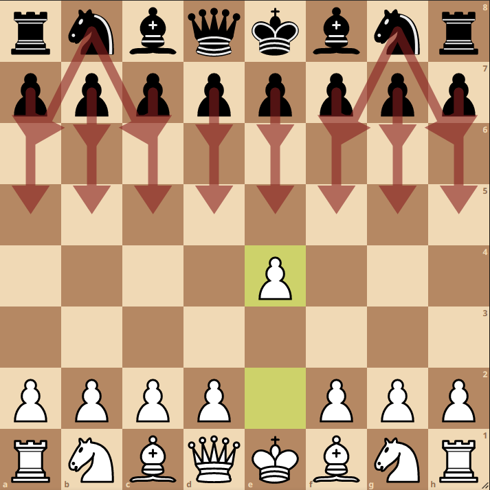 Each board in the particle filter will randomly select one of the available moves, and play that move on its board. After turn 1, the $N$ boards will now approximate the distribution of black pieces on the board. White chooses a location to sense, and receives information about a 3x3 section of the grid. This information will be compared to all boards in the belief state, and boards which do not match the sense will be removed from the belief state.
In the general case, the particle filter is propagated forward by selecting a random move legal for black in RBMC for each board in the belief state, and then pruning the belief state with observations.
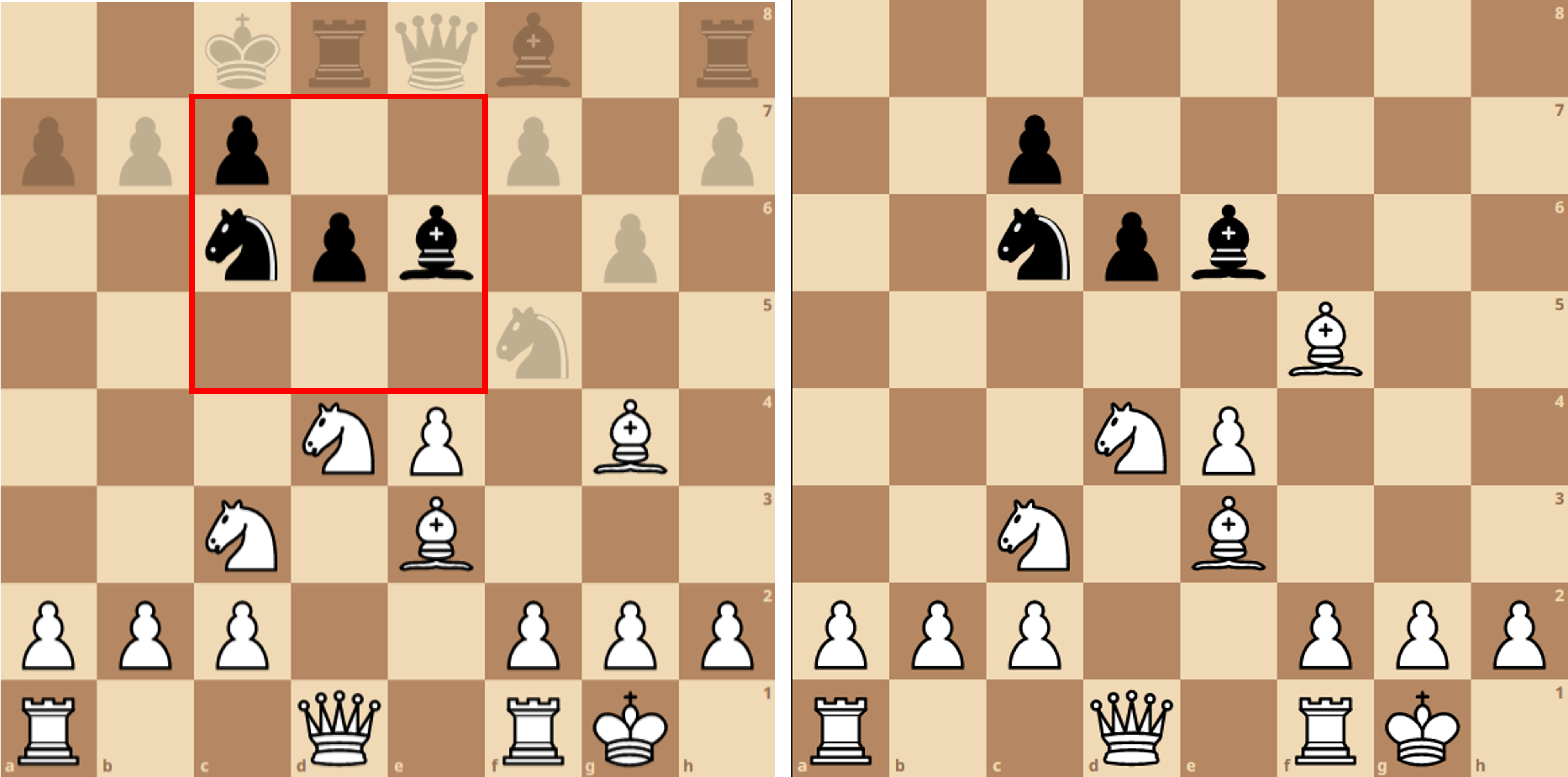
Sensing is only one of three possible observations in RBMC. Information is also gained when the agent makes a move, or when the opponent makes a move. When the agent makes a move, a requested move is sent to the game manager. The game manager returns the taken move, which may differ from the requested move, as explained in the Rules section. The difference between the requested and taken moves (or them being the same) provides information about the board which can be used to remove boards from the particle filter. For instance, assume that white is in the given position, and has sensed on d6, seeing the bishop on e6. White then requests e6, but takes f5. This informs white that a black piece must have occupied f5, and boards where this is not true can be removed.
Similarly, if black captures a white piece, only boards where such a capture was possible need to be retained. If white captures a piece (and is informed only that a piece was captured, not which piece), boards where the captured square was empty can be eliminated.
Two nuances remain in the particle filter’s implementation: resampling to retain $N$ boards once boards are eliminated, and reinitializing the particle filter if an observation contradicts all existing boards.
Resampling Boards
One candidate method of resampling is to simply oversample the remaining boards when selecting the next move for black. While this is simple to implement, it does artificially reduce the variable of the distribution between moves. Instead, I implemented a search algorithm to look 1 move in the past, and look for black moves which would allow the current observation to be generated. This ensures that there are always $N$ boards being sampled from when black’s move is simulated.
For example, say white moved a bishop, and captured a piece short of the requested square, as in the image above. All boards without a piece on f5 are eliminated. Instead of sampling from the remaining boards, the removed boards are replaced by going one move into the past, and sampling boards which have available moves that result in a piece being on f5. This has two advantages: it avoids artificially reducing the particle filter’s variance, and it avoids premature initialization of the particle filter. For instance, if no boards in the belief state had a black piece on f5, the oversampling method would be forced to reinitialize the particle filter. However, if looking 1 move into the past, a move for black can be found on a previous board to place a piece on f5 (which was not selected during the previous simulation step), this move can be used instead of reinitializing the filter.
This process can be improved by looking farther into the past when necessary (I.E. 2+ moves back), at the cost of significant computational time.
Reinitializing the Filter
Even when looking into the past, situations can occur where no boards are able to agree with the observation presented. When this occurs, the particle filter must be reinitialized. This could be done completely randomly, which sacrifices all information gained up the the current state. Instead, my implementation samples pieces from the current boards distribution held in the belief state, plus some uniform randomness (the real board was not in the belief state, so additional randomness is necessary). Additionally, the board is forced to agree with the current observation.
Sensing
The location to sense is determined by balancing information gain with threatening and weak squares within the current board distribution. First, the entropy of each square is computed using: \(H(X) = -\sum_{i\in S}{P(X=i)\log{P(X=i)}}\) Where $H(X)$ is the entropy of square $X$, $S$ is the set of possible states for that square (each type of chess piece for each color, and empty), and $P(X=i)$ is the probability of the square being in specific state, I.E. a4 containing a black rook, where $P(X=i)$ is approximated from the belief state as: \(P(X=i)\approx \frac{1}{N}\sum_{b\in B}b(X)==i\) Where $b$ is a board in the belief state $B$, and $b(X)$ is the state of square $X$ on board $b$.
Similarly, the ‘Threat Value’ $T(X)$ and ‘Weakness Value’ $W(X)$ are computed for each square. The Threat Value of a square is defined as the total material value that the piece on that square attacks, and is only non-zero for opponent pieces. The Weakness Value is defined as the product of a piece’s value and the number of pieces attacking it, and is similarly defined as non-zero for opponent pieces. The Threat and Weakness values are summed over all boards in the belief state.
With these values, the sense operation is chosen to maximize the sum of the heuristic $L$ across the nine squares in the sense region: \(L(X) = \left(T(X) + W(X) + \alpha\right) * H(X)\) Where $\alpha$ is a parameter which weights the priority of maximizing information gain and threat or attack. Multiplying the threat and weakness values by the entropy ensures that these are only prioritized if they are uncertain; squares that have a high degree of certainty don’t need to be sensed.
If $X=(X_r,X_c)$ is defined by its rank and file (row and column), then the sense is chosen: \(X_{sense} = \operatorname*{argmin}_{X}\sum_{r=X_r-1}^{X_r + 1}{\sum_{c=X_c-1}^{X_c + 1}{L(r,c)}}\)
Move Selection
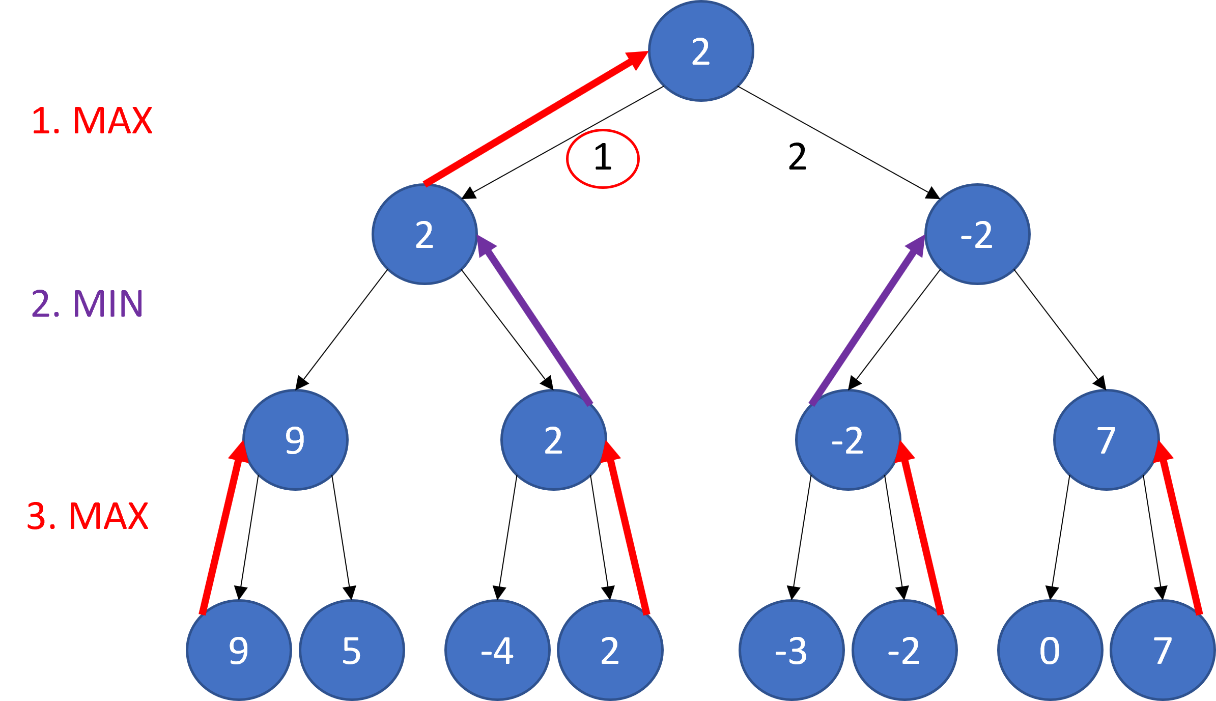
Move selection is performed using Minimax Search with alpha/beta pruning, a well known chess search algorithm. In brief, Minimax search creates a search tree, where an evaluation function is alternately maximized (when it is the agent’s turn) and minimized (when it is the opponent’s turn).
The search tree below creates and exhaustive search tree to depth 3. Starting from the leaf nodes, the evaluation function is alternatively maximized (on the agent’s turn) and minimized (on the opponent’s turn) up the tree. Move one is selected, because this is the move which leads to the best node at the tree’s maximum depth.
 Note that not much search effort can be retained after each move. Chess has a branching factor of around 30.
Alpha/Beta pruning is a method of branch and bound search which can eliminate subtrees from being pursued if a better (or worse, depending on min/max) alternative has already been found.
Two nuances of minimax in this application still require discussion: the evaluation function, and dealing with uncertainty.
Evaluation Function
My first approach to this problem was to train a neural network to approximate Stockfish evaluations of the given board. One branch of the repo has the partial results from this: training a rather large residual network structure obtained and RMSE of ~1.4, indicating that the network was able to evaluate positions within around one and a half pawns of a Stockfish evaluation. While this was a usable result, I was able to obtain a faster evaluation using a handcrafted heuristic, which relied on material count and piece square tables. Material count simply evaluates which side has more valuable pieces. Piece square tables maintain a static efficacy of placing a piece on each square, such that moving a piece to a good square will increase its evaluation, and a bad square will decrease its evaluation.
Dealing with Uncertainty
To deal with uncertainty, $M«N$ boards are selected from the belief state to search over. Minimax search is apply simultaneously to each of these boards, where the evaluation of each node in the search tree is the average of each of the evaluations of the $M$ boards.
The $M$ boards are choses as the most likely boards from the belief state. If the belief state is viewed as a probability distribution, then the likelihood of a board existing is given as: \(P(b)=\prod_{x\in X}{P(x=b(x))}\) The log probability is computed for each of the $N$ boards, and the $M$ boards with the highest log probability are selected for minimax search.
Results
The agent was evaluated against a random agent, and adversarial knight rush agent (which aimed to captured the king with four knight moves), and in competition against other teams in the CS4649 class at Georgia Tech. My agent only lost to one other team’s agent, 1-2 in a best of three. My agent drew black twice, and may have beat the opponent if it has received white twice.
Overall, the project was quite fun to work on. Future directions I find interesting mainly deal with moving away from reliance on existing chess knowledge, and instead attempting to learn RBMC strategy directly. Various approaches, such as Alpha-Zero style techniques are interesting, but require immense compute and time to become effective. Additionally, RBMC provides significant additional difficulties beyond classical chess, mainly due to the partial observability; learned approaches must either represent a belief state explicitly or perhaps implicitly, through a recursive network structure such as an LSTM.