
This post summarizes the content and contributions of my recent paper on zero dynamics policies, accepted and presented at the Control and Decisions Conference held in Milan, Italy in 2024. We first motivate the problem by investigating the difficulty of constructing outputs with stable zero dynamics for underactuated systems, then demonstrate a constructive method for synthesizing these outputs on linear systems, a control methodology we denote a zero dynamics policy. Similarity between the linear and nonlinear system about the equilibrium allows this method to be be applied to nonlinear systems, and we finish by proposing a learning method to construct zero dynamics policies with larger regions of attraction.
The full text of the paper is available from IEEE, or on arXiv.
The presentation, given at CDC 2024, is available .pptx,. .pdf.
Motivation for Zero Dynamics Policies: Stabilizing Underactuated Systems
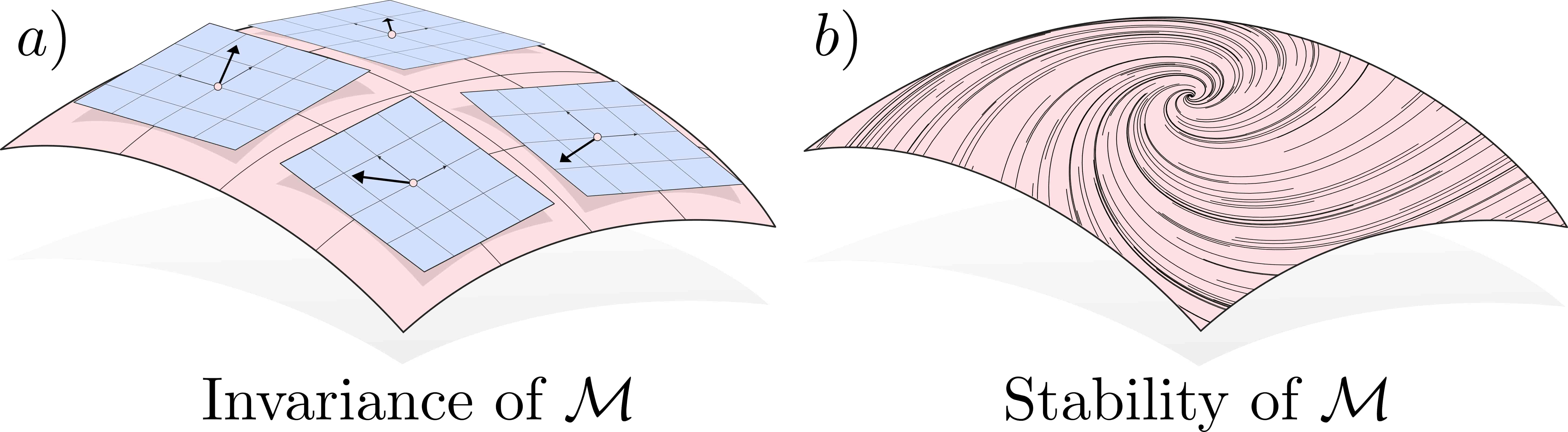
Stabilization of underactuated nonlinear systems is quite challenging from a control theoretic perspective. A deep dive into any book on nonlinear control Sastry, Isidori, will frame nearly all control objectives in terms of driving an output to zero. While a powerful design technique, in general we can only control as many outputs as we have actuators; in the case of underactuated systems, where one or several degrees of freedom are unactuated, we are faced with a problem. After available outputs are zeroed, the remaining degrees of freedom evolve on a manifold, termed the zero dynamics manifold, which is unimpacted by the choice of control. The ‘zero dynamics’ are determined not by choice of controller, but by choice of output - so if a certain set of outputs leads to unstable zero dynamics, the system will be unstable.
The question then becomes, is it possible to construct outputs for a given system which have stable zero dynamics. Up to this point, this question was unanswered for broad classes of systems, including underactuated systems. We prove that locally, underactuated systems are guaranteed to have outputs with stable zero dynamics, and give a constructive method for obtaining these outputs from the linearization of the system about equilibrium. Then, we present a learning problem to find more general outputs which also have stable zero dynamics by construction.
Constructing Zero Dynamics Policies from the Linearization
We start with a core assumption: we assume that the system has an output of valid relative degree (whose zero dynamics are unstable, otherwise we are done). This output describes a coordinate which we have complete control over - we can drive the output to arbitrary (sufficently smooth) trajectories in the state space. This output admist a decomposition of the system into output and normal coordinates (classic result from nonlinear control) which we will term the ‘acutation decomposition’, as it separates coordinates which are actuated from those which are not. Then, we pose the question: given an unactuated coordinate, where is the best possible place for the actuated coordinate to be? This mapping, \(\eta_d = \psi(z)\) implicitly defines a manifold, \(\mathcal{M} = \{\eta, z ~\vert~ \eta = \psi(z)\}\), which can be constructively stabilized by driving the new output \(\eta_1 - \psi_1(z)\) to zero. All that this buys us is the fact that we know that we can constructively stabilize manifolds of this form. However, we still do not know if the zero dynamics on the manifold are stable.
To solve this problem we turn to the linearization of the system (in \(\eta, z\) coordinates). We can stabilize the linearization using LQR or pole placement, and the result is a closed loop stable linear system. Running an eigendecomposition on the \(A_{CL}\) matrix, we can identify eigenspaces of the linear system, which are subspaces which are invariant and have stable dynamics. If we choose a \(\text{dim}(Z)\) dimensional eigenspace of \(A_{CL}\) which is not orthogonal to \(z\) (which we can guarantee exists using tools from linear algebra), then this surface is precisely a manifold which can be parameterized in terms of \(\psi\). Therefore, for the linear system, we have determined an output, \(\eta_1 - \psi_1(z)\), which has stable zero dynamics.
Local Zero Dynamics Policies for Nonlinear Systems via Linearization
If we drive this same output to zero for the nonlinear system, we recover stability in a neighborhood of the origin; this can be shown by leveraging the fact that the nonlinear dynamics cannot change from the linearization too quickly, locally around the origin. This gives us a constructive method for local stabilization of underactuated systems via output stabilization, a tool which did not exist previously.
A critical parallel to this work is the fact that LQR locally stabilizes underactuated systems in a neighborhood of the equilibrium position, Tedrake. This work is tightly coupled to this idea, but reframes it in the context of nonlinear control’s favorite tool, output stabilization.
Learning Zero Dynamics Policies via Optimal Control
To extend these zero dynamics policies away from the origin, we parameterize them as a neural network \(\psi_{\theta}\), with parameters \(\theta\). Then, leveraging the fact that optimal control converges to LQR around the origin, we know that locally, optimal control will exhibit the same controlled invariant manifolds as the LQR solution - the problem is well posed. Additionally, since optimal control is stabilizing (the infinite time integral will not converge if the system does not approach the origin), we simply look for a manifold of the proposed structure which is invariant under the optimal control action. To do this, we minimize a loss which is exactly the current deviation from invariance under the optimal control \(u^*\).
\(\mathcal{L}(\theta) = \mathbb{E}_{z} \left \|\hat{f}(\zeta_{\theta}) + \hat{g}(\zeta_{\theta})u^*(\zeta_{\theta}) - \frac{\partial \psi_{\theta}}{\partial z} \omega(\zeta_{\theta}) \right \|\) where \(\zeta_\theta = (\psi_\theta(z), z)\)
When this loss is driven to zero, the resulting manifold is invariant under the action of the optimal controller, and stable (since the optimal controller is stabilizing), and therefore meets the requirements for a zero dynamics policy. Stablizing the manifold (driving the associated output to zero) stabilizes the entire system.
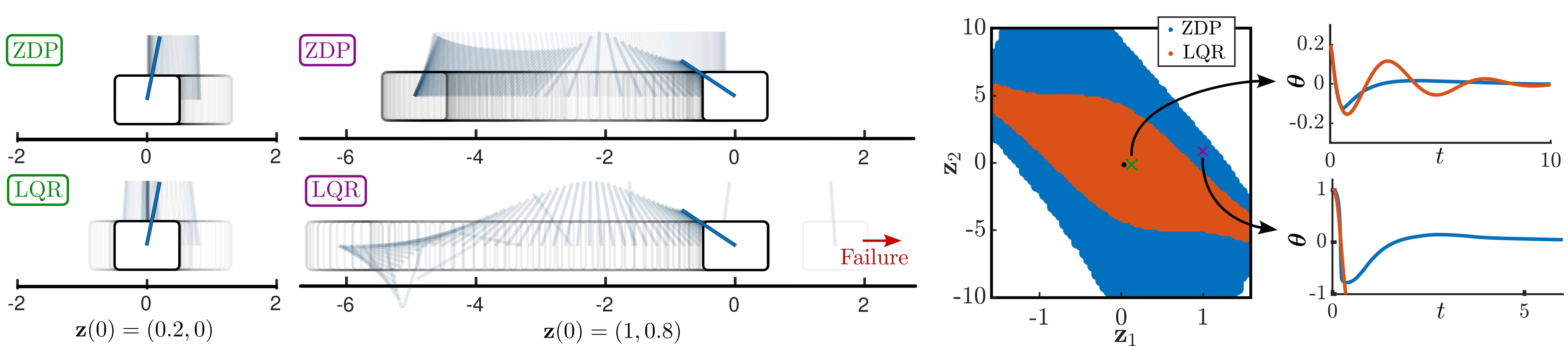
Application to the Cartpole
We deploy this method on the familiar application of the cartpole. The learned zero dynamics policy is able to leverage understanding of the nonlinearities of the system to achieve a larger region of attraction than LQR.
Conclusion
Zero Dynamics Policies (ZDPs) offer a constructive, general method for stabilizing underactuated nonlinear systems by:
- Constructing an output with locally stable zero dynamics from the linearization of the system about equilibrium.
- Explicitly learning a stable, invariant manifold to increase the region of attraction of the zero dynamics policy.
- Separating the design into offline learning (expensive) and online tracking (efficient).
This framework bridges classical nonlinear control and learning-based methods, with promising applications in robotics and beyond. This work is extended to control a particular hybrid system, a hopping robot, in my work on zero dynamics policies for robust agility.