
This post summarizes the content and contributions of my recent paper on Dynamic Tube MPC, accepted and to be presented at the International Conference on Robotics and Automation 2025, in Atlanta, Georgia. We begin by motivating the problem by considering 1) rational of the planner-tracker paradigm and 2) issues with feasibility and conservatism with classical tube MPC. Secondly, we introduce a learning problem, leveraging massively parallel simulation to learn tube dynamics, to optimize collision free trajectories for the system. Finally, we deploy the method on a hopping robot, ARCHER.
The full text paper can be found on arXiv.
Motivating Dynamic Tube MPC: Planner-Tracker Paradigm and Classical Tube MPC
When planning paths in cluttered environments, roboticists have a a few main of tools at thier disposal: graph search methods (including A* on a discrete grid, and RRT to construct a graph, followed by A* to search it), heuristic methods (artificial potential fields, …) and optimization based methods (model predictive control). When the state or dynamics of the robot is complicated, for instance in the case of a humaniod robot or a hopping robot, none of these methods are computationally tractible to solve planning problems; even at a few dimensions, the curse of dimensionality indicates that the space will be too large to search through, and too nonlinear, nonconvex, and long horizon to optimize for. In this case, roboticists will typically turn to a durastically simplified model of the robot to solve the planning problem, typically one of:
- planar state representation $x \in \mathcal{R}^2$, no dynamics (kinematic connectivity only)
- reduced state representation, simple dynamics (single/double integrator, unicycle)
Whatever plan is created using this model representation, called the planning model will then be passed down to a tracking controller, designed to control the tracking model to follow the plan. The planner-tracker paradigm, quite old in robotics, has been treated quite nicely by some of Claire Tomlin’s work. Critically, because the planner and tracker do not share the same dynamics, the tracking model will incur error when it tracks the plan. This error can lead to collisions in the environment, if not accounted for correctly.
The easiest and fastest adjustment to account for the model mismatch is the buffer all of the obstacles in the environment by a heuristic margin. If this margin is large enough, meaning that the true system will stay with a tube of this size around the nominal trajectory, then it will avoid collision with the environment; this approach is known as tube model predictive control (Tube MPC) - or more specifically, Fixed Tube MPC. From a theoretical perspective, if the tracking controller can establish a robust tracking invariant around the nominal trajectory, then planning a trajectory such that the tube, created by buffering the plan by the tracking invariant, lies in the free space gives guaranteed collision free paths.
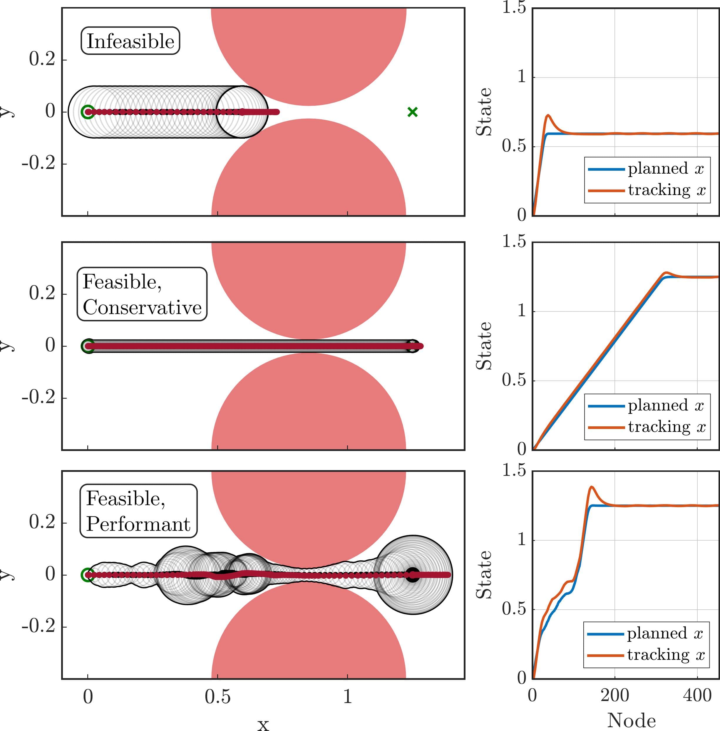
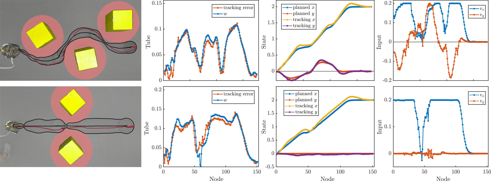
However, fixing the size of the tube a-priori can lead to significant issues, namely overly conservative behaviors, or unecessary infeasibility, as shown in the figure above. Our key insight is the fact that the size of the tracking tube typically depends on the trajectory you are trying to track. For instance, a drone can track a hover point quite well - however, it will incur larger tracking error if you command it to turn a sharp right angle at maximum speed. If I want a tracking invariant for both of these behaviors, it will be as large as the biggest errors collected during the most aggressive manuevers - but this tube is incredibly conservative for less dynamic, slower behaviors. The conservative nature of the tube for slower behaviors can lead to planners either 1) not being able to find a route, or 2) require a large excess of conservative behavior, when an aggressive route to the goal exists.
We propose a method to learn a dynamic representation of the tracking invariant tube, which depends on both a history of previous errors, and information about the plan being tracked. This results in smaller tubes for easier to track paths, and larger tubes for more difficult to track paths. We then integrate this dynamic tube into a Dynamic Tube MPC planner, which generates plans such that the dynamic tube lies is the free space. This leads to behaviors where the robot moves at maximum agility when far from obstacles, but slows down to safely navigate narrow gaps and tight spaces, enabling safe and dynamic navigation of cluttered environments.
Learning Tube Dynamics
To learn the the tube dynamics, we must first defined the planner-tracker paradigm. We take a system model with discrete dynamics
\(\mathbf{x}_{k+1} = \mathbf{f}(\mathbf{x}_k, \mathbf{u}_k)\) and a planning model, typically with significantly simplified dynamics,
\(\mathbf{z}_{k+1} = \mathbf{f}_{\mathbf{z}}(\mathbf{z}_k, \mathbf{v}_k)\) Add a map \(\mathbf{\Pi}\) which takes a full order state and maps it to a state of the planning model. Finally, we assume we have a tracking controller, $\mathbf{u}_k = \mathbf{k}(\mathbf{x}_k, \mathbf{z}_k, \mathbf{v}_k)$, which tracks the planning model trajectory on the tracking model.
To learn the tube dynamics, we collect a large dataset containing trajectories of the planning model, as well as trajectories of the tracking model, under the action of the tracking controller. These datasets take the form \(\mathcal{D} = \{\mathbf{z}_{0:\bar{N}+1}, \mathbf{v}_{0:\bar{N}}, \mathbf{\Pi}(\mathbf{x}_{0:\bar{N}+1})\}\). From this dataset, we train a neural network to predict a tube which the system will stay within around a given planned trajectory. We define the tube dynamics recursively via:
\(w_{j+1} = f_w(\tilde{e}_{j-H:j}, \mathbf{z}_{j-H,j}, \mathbf{v}_{j-H,j})\) where \(w\) is the width of the tube.
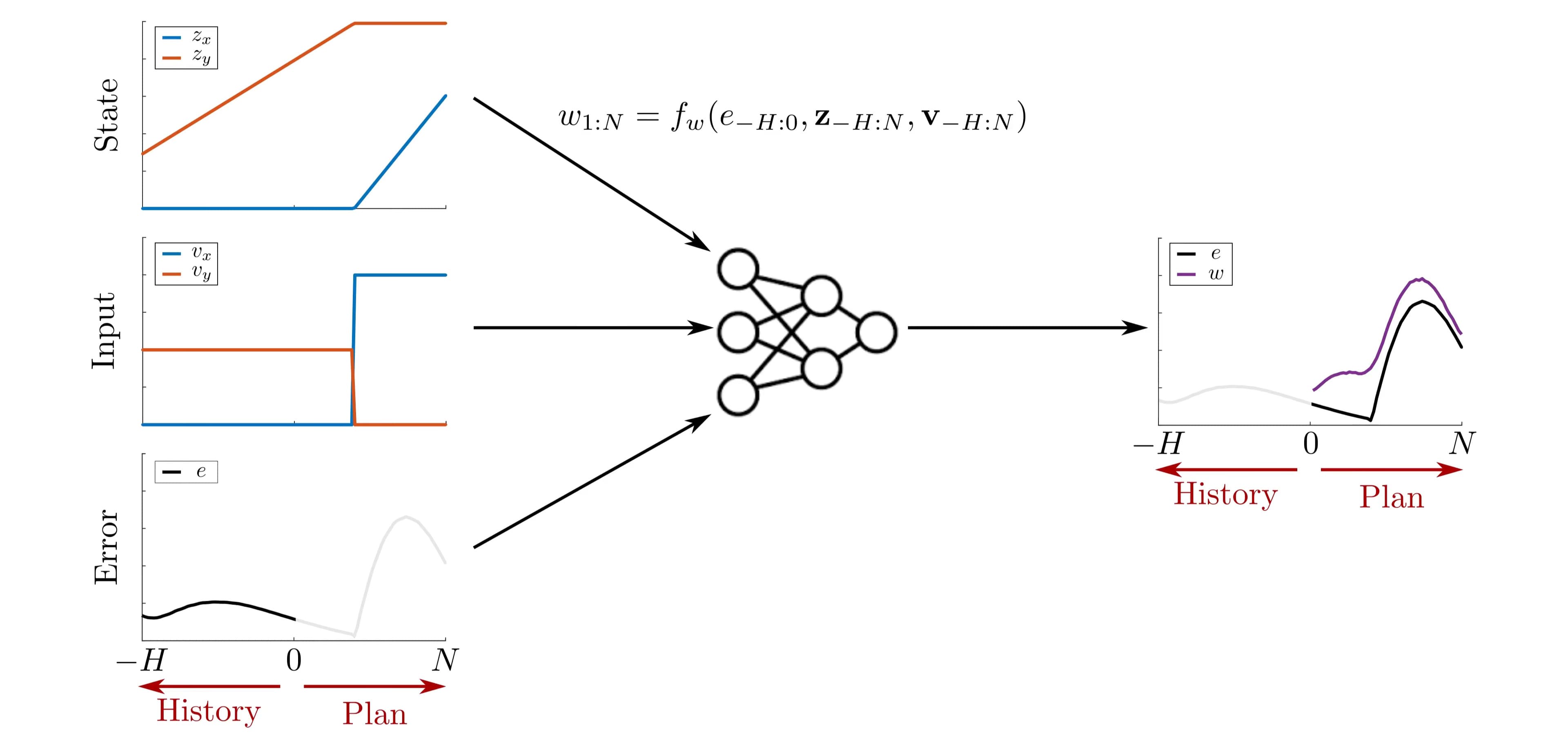
we predict the size of the next tube from the previous system errors, \(e_k = \|\mathbf{z}_k - \mathbf{\Pi}(\mathbf{x}_k)\|\) as well as the previous planned trajectory. We parameterize these tube dynamics via a neural network with parameters \(\mathbf{\theta}\), denoted \(\mathbf{f}_w^{\mathbf{\theta}}\), and train the tube dynamics by minimizing a check loss function (see paper for details).
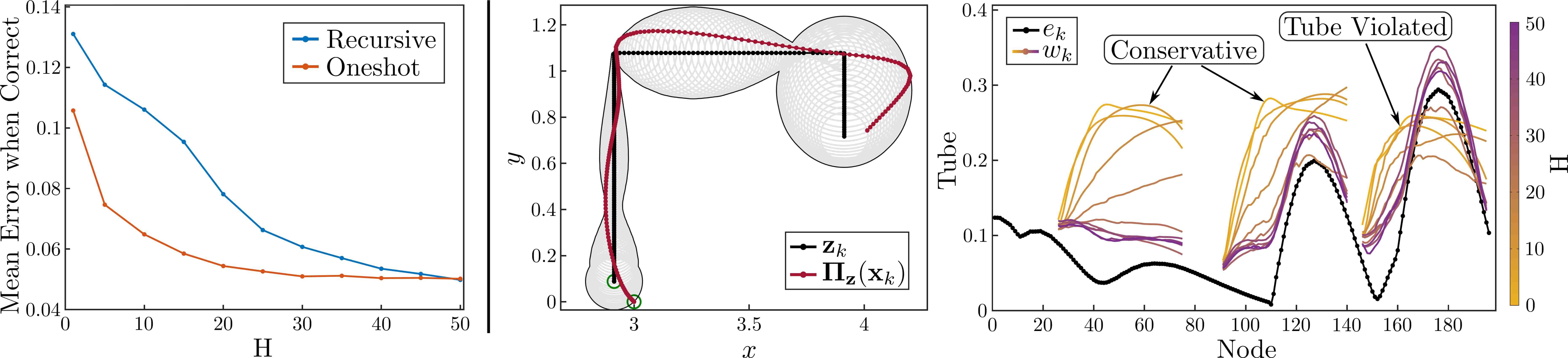
A critical component of this process is the history incorporated into the tube prediction. Without a history, it is very difficult to predict size of the next error with any accuracy: imagine a planning model which only contains positions as states. If we only know the current error, without knowledge of the velocity of the robot, we cannot tell whether this error is increasing or decreasing. A reasonable question, therefore, is why the tube dynamics don’t depend on the tracking model system state, \(\mathbf{x}\). This is to facilitate planning - as seen in the next section, we will use the tube dynamics to plan into the future, using MPC, on only the planning model. As future plans will not included planned states for \(\mathbf{x}\), our tube dynamics cannot depend on them either. However, including a history allows the tube model to effectively filter out relevant information regarding the full order model, and better predict future errors. The effect of the history length is shown in the Figure above, where prediction accuracy monotonically improves with longer history. As longer histories lead to more complex Dynamic Tube MPC problems, we will typically use as short a history as possible to achieve adaquate performance.
Dynamic Tube MPC
With the tube dynamics trained, we simply add our dynamic tube to the classical tube MPC problem:
[
\begin{align}
\inf_{\mathbf{v}{(\cdot)}} J(\mathbf{z}{(\cdot)}, \mathbf{v}{(\cdot)}) &= \mathbf{f}(\mathbf{x}_k, \mathbf{u}_k)
\mathbf{z}{j+1} &= \mathbf{f}{z}(\mathbf{z}_j, \mathbf{v}_j) \quad j \in [0, N-1]
w{0:N} &=f_{w}^{\mathbf \theta}(e_{\,\text{-}H:0}, \mathbf{z}{\,\text{-}H:N}, \mathbf{v}{\,\text{-}H:N})
\mathbf{z}0 &= \mathbf{z}{IC}
\mathbf{v}j &\in \mathcal{V}
B{w_j}(\mathbf{z}_j) &\in \mathcal{C}
\end{align}
]
Where \(J\) is the cost function to be minimized, the first constraint is the planner dynamics, the second the tube dynamics, the third the initial condition, fourth planning input constraints, and last requiring that the tube lie in the free space \(\mathcal{C}\).
Deployment on the ARCHER Platform
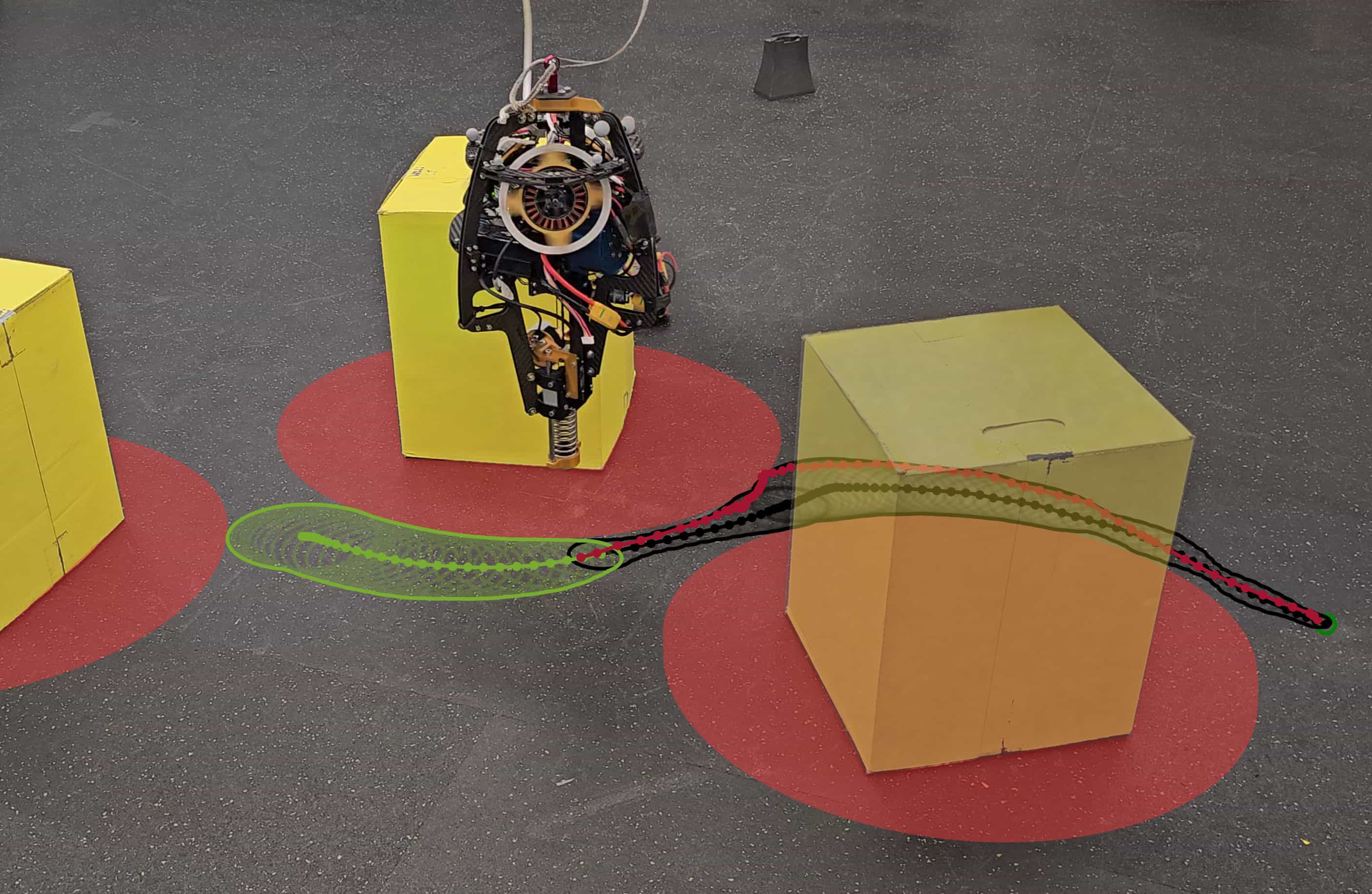
We deploy this dynamic tube MPC on the hopping robot ARCHER. The data to train the tube dynamics is collected using massively parallel simulation in IsaacGym (now IsaacLab!), allowing for millions of transitions to be collected in minutes.
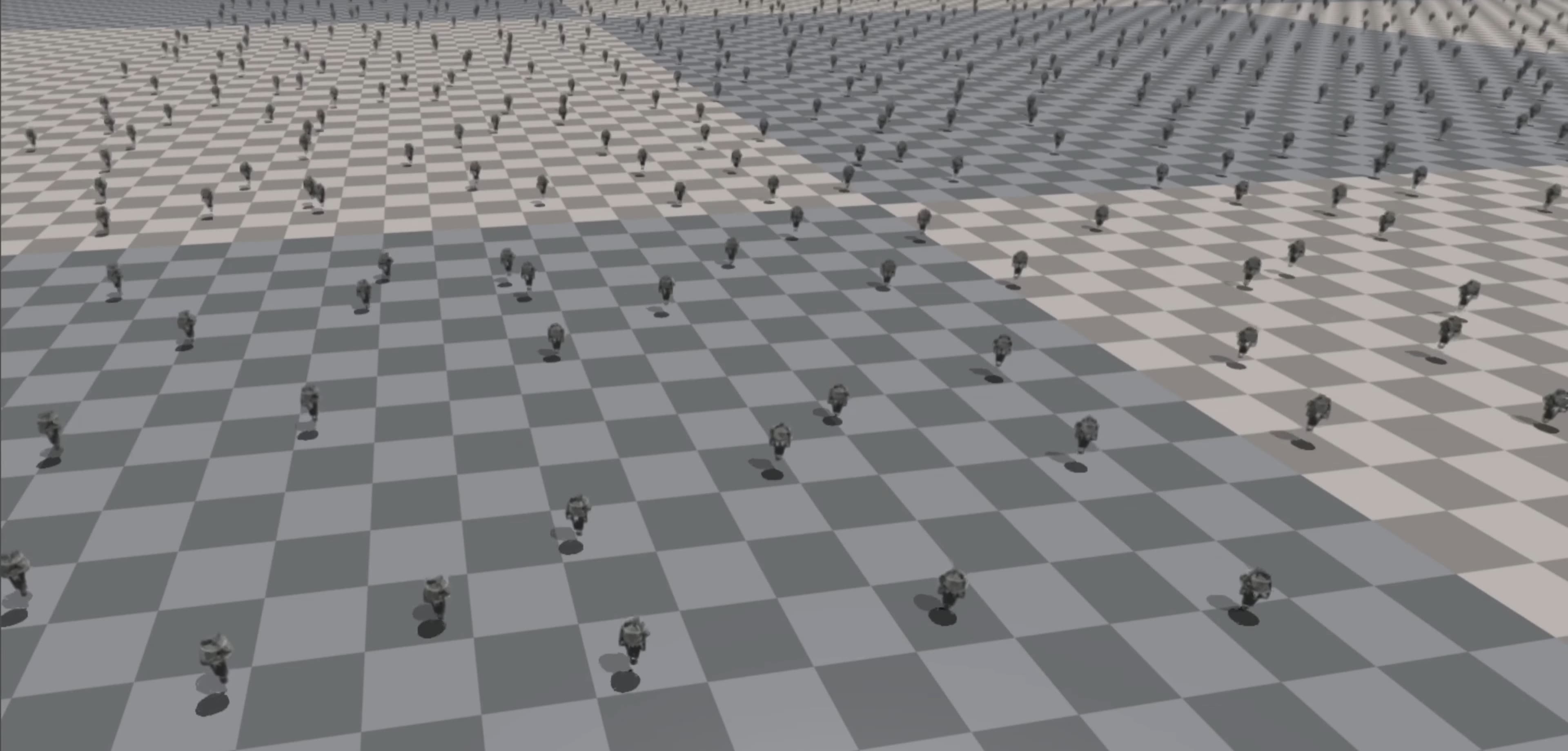
Additionally, this scale of data collection enables domain randomization, which aids in ensuring the tubes trained in simulation will encapuslate the actual dynamics of the hardware system (i.e., addressing the sim2real gap). We deploy the algorithm successfully on the hopper, and observe emergent behaviors where the hopper moves at maximum speed away from obstacles, then reduces its speed to improve tracking near obstacles.
This behavior balances dynamic behaviors with safe navigation of cluttered spaces, on a complex robotic system. A video showcasing the Dynamic Tube MPC on ARCHER is embedded at the top of the page. For other projects involving this awesome hopping robot, see my work on Zero Dynamics Policies (video) and Predictive Control Barrier Functions (video).
Conclusion
Dynamic Tube MPC offers a powerful new framework for safe and agile robot navigation:
- Leverages massively parallel simulation and error histories to learn tracking error tubes which depend on the planned model.
- Formulated an optimization problem which trades off performance and safety in real-time, enabling dynamic and safe behaviors.
- Deploys Dynamic Tube MPC a complex robotic system, the hopping robot ARCHER.