Learning Safe Humanoid Navigation from Reduced Order Models

Abstract

Research in humanoid robotics has achieved rapid progress in locomotion, and recent results have pushed the boundary on autonomous navigation. We demonstrate that a standard single-stage RL navigation pipeline struggles to scale to multi-level and multi-story terrain, limited by the difficulty of complex humanoid terrain interactions such as stairs.

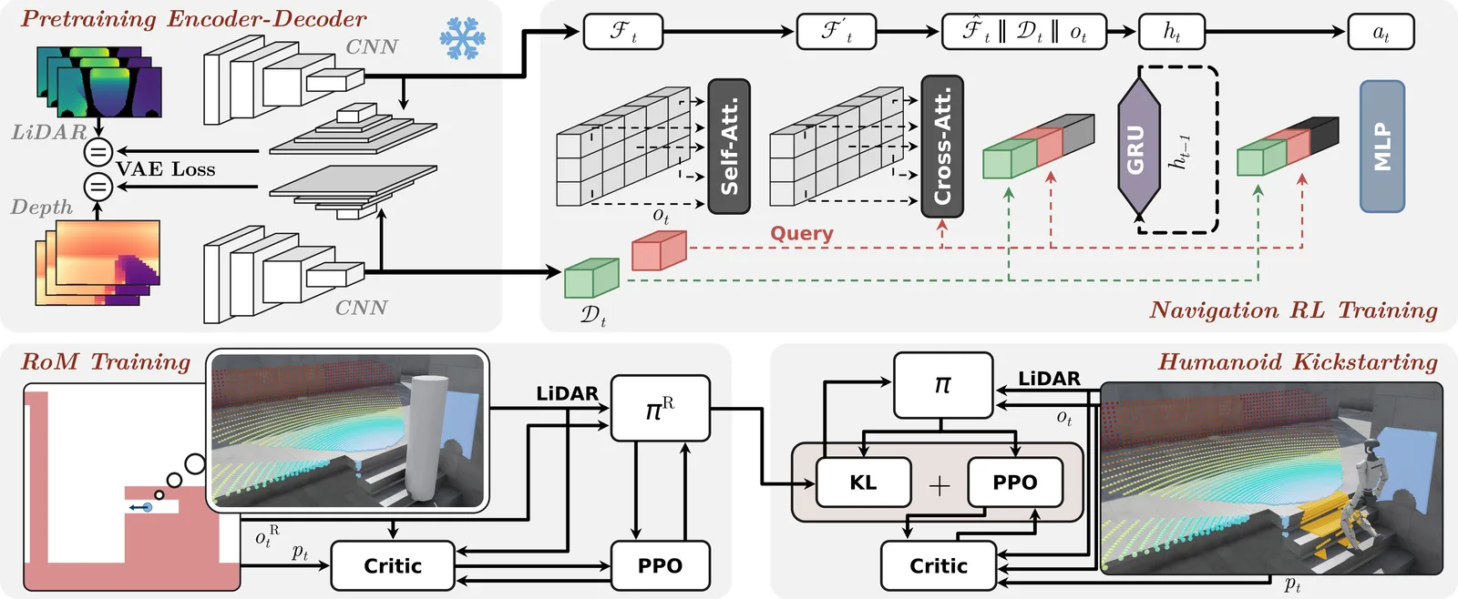
To overcome this challenge, we decompose the navigation problem into two pieces. First, we train a policy operating on the reduced order dynamics but with full 3D LiDAR observations to navigate complex, multi-story terrain. We then utilize this navigation knowledge to kickstart a policy operating on the full-order humanoid dynamics, with a frozen locomotion policy in the loop.

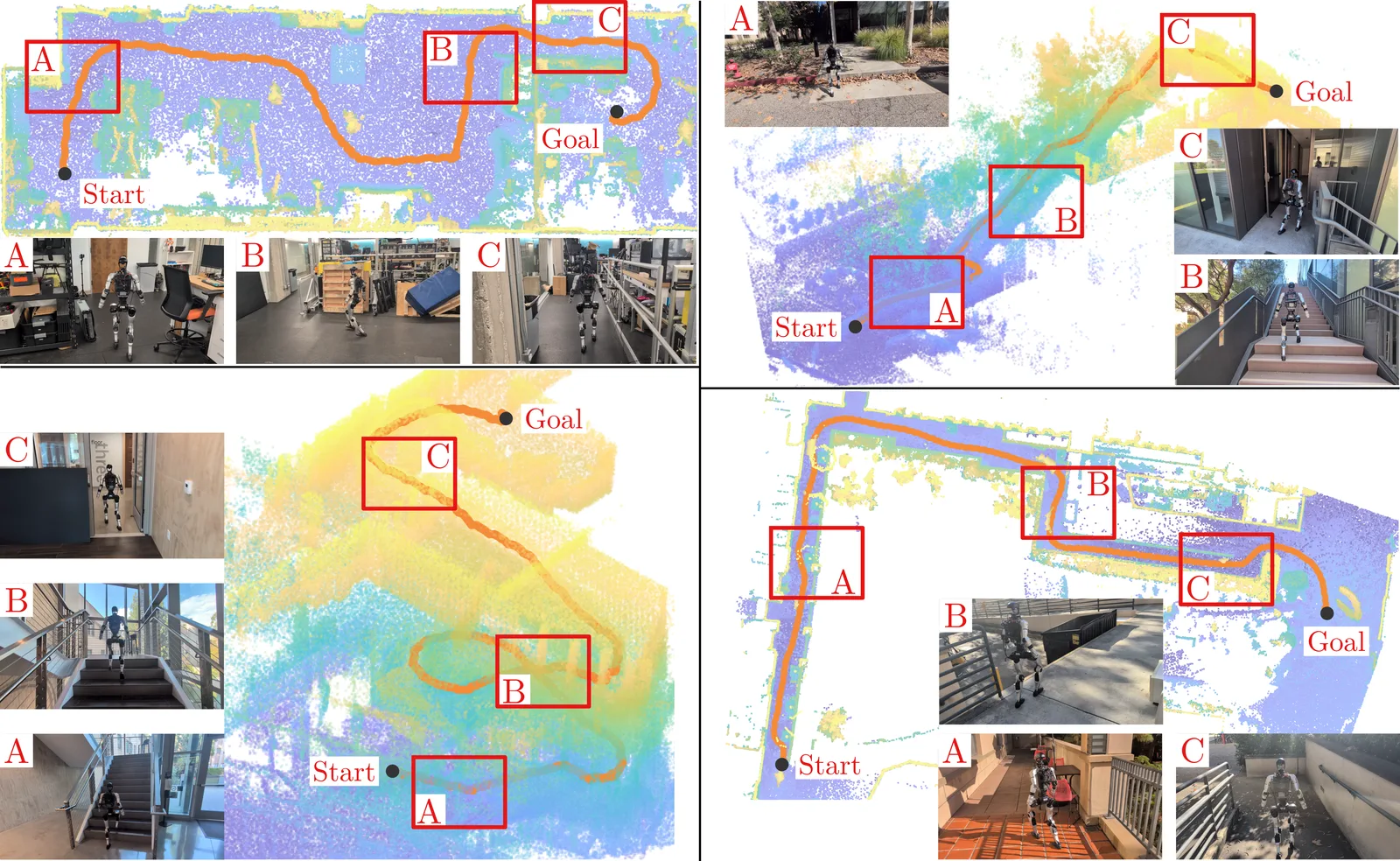
Additionally, we demonstrate that applying a Poisson safety filter to the navigation policy output recovers safety in the presence of out-of-distribution obstacles, without dropping navigation success rate. We demonstrate the resulting RoM-Nav policy on a Unitree G1, accomplishing mapless multi-floor navigation covering trials with over 10 m of vertical displacement and over 100 m of path length.

Method

The navigation policy is trained for deployment on a Unitree G1 equipped with a Mid-360 LiDAR and a downward-facing ZED Mini depth camera. It runs at 5 Hz and emits planar velocity commands to a frozen locomotion policy running at 50 Hz, with limits of 1 m/s forward, 0.25 m/s lateral and 1 rad/s angular.

RoM-Nav architecture: LiDAR and depth encoders feed self- and cross-attention, then a GRU and an MLP head; below, a RoM policy kickstarts the humanoid policy. — **Fig. 2.** RoM-Nav architecture. LiDAR and Depth inputs are processed via a pretrained CNN encoder. LiDAR passes through self- then cross-attention. The resulting embeddings are processed by a GRU unit and mapped to actions via an MLP head. A RoM policy is trained first, which is then used to kickstart the RoM-Nav policy by balancing KL divergence with a PPO objective on the humanoid with frozen locomotion controller. Enlarge.

A.Kickstarting from a reduced order model

The final navigation policy is kickstarted from one trained on a single integrator with heading, whose environment is an occupancy grid derived from the same 3D terrain. When a command drives into an occupied cell, the penetrating component is projected out, sliding along the boundary. Trivializing the environment interaction this way lets the reduced-order policy reach strong navigation performance quickly.

That policy then supervises training on the humanoid through a weighted combination of the PPO objective and a KL divergence against the RoM policy:

$$\mathcal{L} = \mathcal{L}_{\mathrm{PPO}} + \lambda\,\mathcal{L}_{\mathrm{KL}}(\pi, \pi^{R}).$$

The weight $\lambda$ is 1 for the first 100 iterations, then decays to 0.05 by iteration 1100, where it holds until training finishes at 2000 iterations. The RoM policy trains in 12 hours on one H100; the RoM-Nav policy takes 32 hours. Combined training is under 45 hours on a single GPU.

Stage 1. The reduced order model — a single integrator with heading, colliding against the tile's occupancy grid.

Stage 2. The kickstarted humanoid, on the same tile under the same camera, driving a frozen locomotion controller.

B.Pretrained vision encoders

The LiDAR range image and depth image are high-dimensional inputs requiring significant visual processing. Rather than learn these features during RL, we pretrain a CNN encoder for each as a denoising VAE, with heads for depth, XYZ and valid-mask reconstruction plus ground/obstacle/stair/ramp segmentation, so that critical features are retained in the latent. Inputs are noised, 0–80 % pixel dropout is applied, and the robot's head occlusion mask is varied. The encoders are trained for 10 epochs on 1M uniform and 1M stair- and ramp-oversampled images, then frozen.

C.Environments, spawns and goals

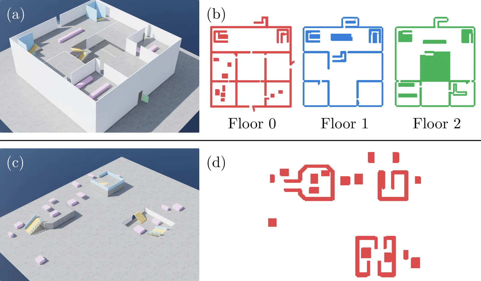
Where existing work uses single-level layouts, deploying in multi-level real-world environments requires a different approach. We procedurally generate outdoor tiles, single-room tiles and multi-story building tiles. A tile is multi-story if there exist $$x, y$$ coordinates containing multiple disjoint $$z$$ locations that are coherent goals — the same planar position on different floors. Because tiles are generated programmatically, ground-truth traversability is recorded during generation and rasterized into a 0.2 m occupancy grid, maintained per floor.

Spawns and goals are not uniform. With probability 0.3 the spawn is placed on or near the mouth of a stair or ramp, drawn from a phase-indexed gait library of the locomotion policy traversing that geometry, so the robot begins mid-stride rather than standing. Goals are capped at 30 m of geodesic distance — computed by a CUDA wavefront kernel — and biased to cross height levels: three-story tiles sample cross-level goals 100 % of the time, other tiles 50 %.

Procedurally generated tiles and their occupancy grids: a multi-story building and a multi-level outdoor environment. — **Fig. 3.** Environment tiles. (a) multi-story building and (b) its occupancy grid. (c) multi-level outdoor environment and (d) its occupancy grid. Enlarge.

III

Results in Simulation

A.RoM kickstarting

We compare four arms. Single-Stage is trained directly on the humanoid via PPO for 4000 iterations. RoM (cyl) is the reduced-order policy evaluated on its own dynamics, an upper bound for the method. RoM (hum) is that same policy deployed zero-shot onto the humanoid. RoM-Nav is the proposed method. Every policy is spawned from the same 1024 initial conditions on terrain generated with a different seed from training.

**Table II.** Navigation performance across training methods. SR@45 / SR@120 are success within 45 s (the training budget) and 120 s; T2G is mean time to reach the goal over successful episodes; SPL is success weighted by path length against the geodesic route. **Bold** marks the best humanoid arm per column. ^*RoM (cyl) is evaluated on RoM dynamics.
Arm	SR@45 (%)	SR@120 (%)	T2G (s)	SPL
RoM (cyl)^*	84.1	93.6	25.6	0.776
Single-Stage	62.2	81.7	32.1	0.690
RoM (hum)	74.2	88.1	29.8	0.713
RoM-Nav	82.3	92.8	28.8	0.769

Single-Stage underperforms throughout, while RoM-Nav lands within 1–2 % of the reduced-order upper bound. The RoM transfers onto the humanoid reasonably well without kickstarting, but kickstarting recovers a further 8 % success at 45 s and 5 % at 120 s.

Three arms, one three-story tile. Left to right: Single-Stage (blue, labeled Nominal on screen), RoM (hum) (red) and RoM-Nav (green), released from a shared initial condition and followed by the same camera. Single-Stage loses the route; the raw RoM transfer fails on the stairs; only RoM-Nav reaches the goal. The divergence is a stair problem, not a walking problem — which is what the paired contrast below isolates.

**Table III.** Success rate paired contrasts by same-level vs. cross-level goals. Positive favors RoM-Nav; ^† marks a 95 % confidence interval excluding zero.
	45 s		120 s
Contrast (%)	same	cross	same	cross
RoM-Nav − RoM (hum)	+1.5	+15.2^†	+0.6	+9.1^†
RoM-Nav − Single-Stage	+6.8^†	+34.6^†	+3.0^†	+19.7^†

RoM-Nav makes all of its progress back on the cross-level trials, where stairs or ramps must be traversed to change $$z$$ level. The improvement comes primarily from fewer falls: on the 120 s cross-level trials, timeout rates are 4.9 % for RoM (hum) against 3.7 % for RoM-Nav, but the fall rate drops from 16.3 % to 8.3 %.

B.Pretrained encoders

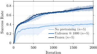
Three variants isolate the encoder choice. No pretraining randomly initializes the CNN and trains it with PPO. Unfrozen @ 1000 takes the pretrained weights and unfreezes them after 1000 iterations. Frozen is the deployed configuration. Without pretraining, success is dramatically reduced; frozen and unfrozen reach equivalent performance, and training the CNN weights costs 15 % more per iteration.

Success rate against training iteration for three LiDAR encoder pretraining variants, mean over five seeds with min-max shading. — **Fig. 4.** An evaluation of the LiDAR encoder pretraining. Success rate vs. training iteration is plotted for three pretraining variations; mean over five random seeds, min-max shaded.

C.Spawn and goal sampling

We ablate the two devices that shape the training distribution: Uniform drops the stair oversampling, NoCap replaces the geodesic goal cap with a Euclidean one, and UniformNoCap drops both.

**Table IV.** Spawn/goal-distribution ablation on the RoM. Metrics identical to Table II. **Bold** marks the best arm per column (T2G excluded, as this metric skews when only short episodes are completed).
Arm	SR@45 (%)	SR@120 (%)	T2G (s)	SPL
RoM	84.1	93.6	25.6	0.776
Uniform	70.9	77.4	23.3	0.640
NoCap	69.8	75.8	22.9	0.624
UniformNoCap	65.7	75.1	24.9	0.601

**Table V.** Spawn/goal pair success rate by same-level vs. cross-level goals. Positive favors RoM; ^† marks a 95 % confidence interval excluding zero.
	45 s		120 s
Contrast (%)	same	cross	same	cross
RoM − Uniform	+0.0	+27.8^†	+0.6	+33.5^†
RoM − NoCap	−0.6	+30.7^†	−0.2	+37.7^†
RoM − UniformNoCap	+1.0	+37.7^†	+0.0	+39.0^†

Removing either device costs significantly and by approximately the same amount, and removing both costs more. The entire loss falls on cross-level goals — the same-level columns are flat to within a point. Both sampling procedures are what make cross-floor navigation learnable.

Safety under Out-of-Distribution Obstacles

A learned navigation policy carries no collision guarantee. We layer a Poisson safety filter on its output: the point cloud is rasterized into a 0.05 m occupancy grid with the ground removed, convolved with the robot's radius, and Poisson's equation is solved over the grid to synthesize a control barrier function $$h$$ directly from raw occupancy — with no learned value function, disturbance model or obstacle detector. A closed-form QP then projects the policy's command onto the safe set:

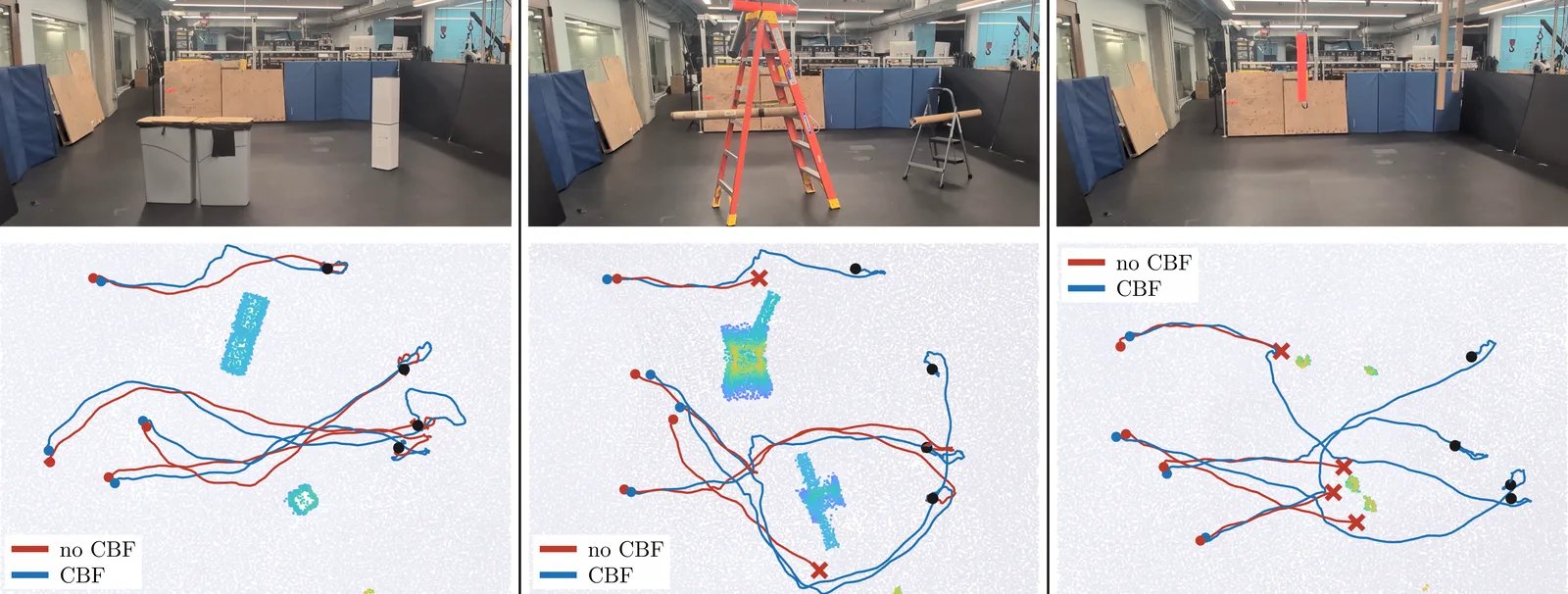
$$v_{\mathrm{safe}} = \arg\inf_{v}\ \lVert v - v_{\mathrm{des}}\rVert^{2} \quad \text{s.t.} \quad \left.\frac{dh}{dp}\right|_{p} v \ \geq\ -\alpha h(p),$$

with $\alpha = 0.75$ . To test it, we built three hardware environments and flew ten shared spawn/goal pairs through each, with the filter both on and off. The room is mapped with GLIM and the robot continuously relocalized, purely to align initial conditions — the map is never available to the policy, which remains strictly mapless.

filter off (left) | filter on (right)

In-distribution. Solid, convex obstacles of the kind the policy trained against. Neither arm collides.

**Table VI.** Hardware CBF comparison in three environments. Initial conditions and goals are shared across arms and environments.
Obstacle Type	Arm	Success	Collision(s)	Time to goal (s)
In-Distribution	no CBF	10/10	0/10	5.9 ± 1.5
	CBF	10/10	0/10	6.7 ± 2.1
Out-of-Distribution	no CBF	10/10	2/10	7.5 ± 1.7
	CBF	10/10	0/10	11.0 ± 5.8
Adversarial	no CBF	10/10	4/10	5.5 ± 1.0
	CBF	10/10	0/10	6.9 ± 1.7

On in-distribution obstacles neither arm collides. On out-of-distribution geometry the unfiltered policy collides twice, and on the adversarial hanging tubes four times; the filter collides on neither. It pays for this in time to goal, which rises in both out-of-distribution environments. Success rate never drops.

Trajectory plots for the three obstacle environments, with collisions marked. — **Fig. 5.** Investigation on performance with OOD obstacles. Four of ten trials are plotted (collisions marked with ×). (Left) Environment with in-distribution obstacles. (Middle) Environment with OOD obstacles. (Right) Environment with obstacles chosen adversarially, hanging with small LiDAR cross-section. Enlarge.

Hardware Deployment

We deploy RoM-Nav on a Unitree G1 for mapless, long-horizon navigation in real buildings and outdoors. The trials include vertical climbs of up to 10 m — beyond the training distribution extreme of 8 m — and path lengths of up to 100 m, well beyond the 30 m training cap. None of the hardware trials included a collision.

Each composite below shows the third-person view alongside the registered LiDAR map with the walked route, the live LiDAR return, and the robot's own depth camera. Figures quoted are measured from each run's recorded bag.

Cluttered lab. 36.6 m of path over 63 s, threading mats, crates and equipment on a single level. Stops 0.03 m from the commanded goal.

Four hardware deployments plotted as registered maps with the walked route. — **Fig. 6.** Four example deployments in complex, real-world environments. (Top Left) Navigation of a cluttered lab environment, 38 m path length. (Top Right) 2-Story climb (7 m ascent) on a wire-railed stairwell, 51 m path length. (Bottom Left) 2-Story climb (10 m ascent) to enter a building from the outside, 51 m path length. (Bottom Right) A long-horizon outdoor navigation task, avoiding tables, cliff edges and railings, 100 m path length (1 m descent). *Panels are plotted from separate recorded runs; the videos above are their own takes.* Enlarge.

Limitations

LiDAR is not a sufficient sensor for transparent obstacles: a cardboard sheet was used to block a glass door and window in one trial, which the robot might otherwise have tried to traverse. Beyond those specific instances, no intentional environmental modifications were required. The method also assumes an accurate goal expressed in the body frame, which is a strong assumption. Finally, the planar CBF could in principle block routes the policy deems traversable, though this was not observed experimentally.

Supplementary Video

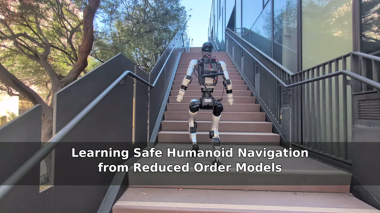
The full supplementary video covers the architecture, both training stages, the policy comparison in simulation, the safety filter, and all four hardware deployments at length.

Play · 8:36

—

Citation

BibTeX

@misc{romnav2026,
  title         = {Learning Safe Humanoid Navigation from Reduced Order Models},
  author        = {Compton, William D. and Olkin, Zachary and Bena, Ryan and Ames, Aaron D.},
  year          = {2026},
  eprint        = {TODO},
  archivePrefix = {arXiv},
  primaryClass  = {cs.RO}
}